Teaching Talk

class: center, middle, inverse, title-slide

# Teaching Talk
### Colin Rundel Duke University
### University of Edinburgh - 2018

---

exclude: true

---

## Melanism in Peppered Moths

.pull-left[
<img src="imgs/typica.jpg" width="693" /><img src="imgs/carbonaria.jpg" width="693" />
]

.pull-right[
* *Biston betularia* is a common and widely spread (Asia, Europe, & N. America) species of moth

* The species exhibits several different naturally occurring (and genetically determined) colorations

- The lightly colored (above) is referred to as *typica*
    
    - The darkly colored (below) is referred to as *carbonaria*
    
* Put forward as an example of evolution by natural selection (different predation rates)
]

.footnote[
Photos by [Olaf Leillinger](https://de.wikipedia.org/wiki/User:olei) via [Wikipedia](https://en.wikipedia.org/wiki/Peppered_moth_evolution).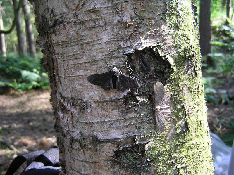
]

---

![](imgs/tree.jpg)

.footnote[
Photo by [Martinowksy](https://nl.wikipedia.org/wiki/User:Martinowksy) via [Wikipedia](https://en.wikipedia.org/wiki/Peppered_moth_evolution).
]

---

## Example

Assume that a researcher is interested in understanding the different rates of predation under differing environmental conditions. As a pilot study, they contaminate a small aviary with soot by burning coal and then releasing a large but equal number of *typica* and *carbonaria* peppered moths into the enclosure.

After several days, the researcher then introduces a small number of insectivorous birds (known to eat the moths) into the aviary.

Finally, after two days of exposure to the predators the research returns to the aviary and collects a sample of the remaining moths. Within their sample they find:

.center[
| Form         | Count |
|:-------------|-------|
| *typica*     |  12   |
| *carbonaria* |  31   |
]

---

## A data model

Is there a simple probabilistic model that we can use to represent the generative process for these data?

What if instead of moths in an aviary we instead thought of marbles in an urn?

Based on our model choice, what is the parameter of interest? What does its value tell us in the context of the experiment?

Are there any assumptions that we are making when we choose this model?

---

## Likelihood, Prior, ...

We have chosen a binomial distribution as our *likelihood* model for our data,
$$ Y \sim Binom(n=43, p) $$
where `$Y$` is the number of carbonaria moths sampled.

For this example, we will choose to represent our *prior* beliefs about the parameter `$p$`, the proportion of surviving carbonaria moths, using a beta distribution with shape parameters `$a$` and `$b$`.
$$ p \sim Beta(a,b) $$

Our ultimate goal is inference, we would like to use our *likelihood* and the *prior* to be able to say something useful about the distribution of `$p$` given our observed data,
$$ p | Y = 31 \sim ~?. $$
This is the *posterior* distribution for our parameter of interest which we can construct using Bayes' theorem.

---

## Bayes Theorem

Likelihood:
`\begin{align}
Y& \sim Binom(n=43, p) \\
P(Y&=y|p,n) = \frac{n!}{y!(n-y)!}p^y(1-p)^{n-y}
\end{align}`

Prior:
`\begin{align}
p& \sim Beta(a,b) \\
f(p&|a,b) = \frac{\Gamma(a) \, \Gamma(B)}{\Gamma(a+b)} p^{a-1}\,(1-p)^{b-1}
\end{align}`

Bayes' theorem:
`\begin{align}
f(p|Y=y) 
  &= \frac{P(Y=y|p)}{P(Y=y)}f(p) \\
  &= \frac{P(Y=y|p)}{\int_0^1 P(Y=y|p)\,f(p)\,dp}f(p)
\end{align}`

---

## Derivation

`\begin{align}
f(p|Y=y) 
  &\propto P(Y=y|p)\,f(p) \\~\\
  &\propto \left( \frac{n!}{y!(n-y)!}p^y(1-p)^{n-y} \right)
           \left( \frac{\Gamma(a) \, \Gamma(B)}{\Gamma(a+b)} p^{a-1}\,(1-p)^{b-1} \right) \\~\\
  &\propto \left( p^y \, (1-p)^{n-y} \right)
           \left( p^{a-1} \, (1-p)^{b-1} \right) \\~\\
  &\propto p^{a+y-1} \, (1-p)^{b+n-y-1}
\end{align}`

$$ p|Y=y \sim Beta(a+y, b+n-y) $$

---

## Lets explore

.medium[.center[

[http://bit.ly/ed2018_betabinom](http://bit.ly/ed2018_betabinom)

]]

---

## Credible intervals

The intervals we found for `$p$` are called credible intervals, like confidence intervals they allow us to conduct inference on our parameter of interest.

Some important characteristics of credible intervals,

* depend on *both* the data and the prior

* allow for direct probabilistic statements about the parameter

* do not depend on large sample theory or any kind of normal approximation.

* are not unique for a given posterior distribution
  - in the shiny app they are determined by requiring that the probability mass in the upper and lower tails be equal.

---
count: false

## Review - Beta distribution

Let `$X$` be a random variable with a `$beta(a,b)$` distribution with shape parameters `$a$` and `$b$` then,

.pull-left[

$$ f(x | a, b) = \frac{\Gamma(a) \, \Gamma(B)}{\Gamma(a+b)} x^{a-1}\,(1-x)^{b-1} $$

for `$x \in [0,1]$`, `$a>0$`, and `$b>0$`.

]

.pull-right[
$$ E(X) = \frac{a}{a+b} $$

$$ Var(X) = \frac{ab}{(a+b)^2(a+b+1)} $$
]